14 Functional Module Identification
This chapter describes how to identify functional modules using the MAPA Shiny application. The Shiny web app provides an intuitive interface for clustering similar pathways into functional modules and assessing clustering quality.
Prerequisites: Before identifying functional modules, ensure you have either:
- Completed pathway similarity calculation in the current session using the Pathway Similarity section as described in the previous chapter, OR
- Upload existing similarity results using the file upload option at the top of the interface.
The similarity calculation results are required for functional module identification to proceed.
14.1 Overview
The Module Identification section in the MAPA Shiny web app lets you run clustering directly on the pathway similarity matrix and then assess clustering quality with built-in diagnostics.
This two-step flow (cluster → assess quality) helps you produce biologically meaningful pathway modules.
14.2 Step 1: Load Your Data
Option 1: Continue from Previous Step
If you have completed pathway similarity calculation in the current session, your data will automatically be available for module identification.
Option 2: Upload Existing Results
If you have previously saved similarity results, you can upload them:
- Click “Browse” at the top of the left panel “Upload Similarity Result (.rda)” to upload your similarity results file (.rda format)
- Select your file
- Wait for validation - the app will automatically detect the input type and prepare for Module Identification.
14.3 Step 2: Perform Module Identification
Set parameters:
Similarity cutoff: Controls the sparsity/cut level used by the selected method. Smaller values generally retain more edges and yield larger modules; larger values retain fewer edges and yield smaller modules. (Exact behavior varies by algorithm.)
Clustering method: Choose from the available methods in the dropdown.
Hierarchical linkage (shown only when a hierarchical method is selected): Choose the agglomeration linkage.
Click “Submit” to run Module Identification.
Monitor progress clustering typically completes within minutes
Review results under “Module identification result” (Table / Data visualization / R object).
14.4 Step 3: Review Module Identification Results
After clustering finishes, examine your results in “Module identification result” with three sub-tabs:
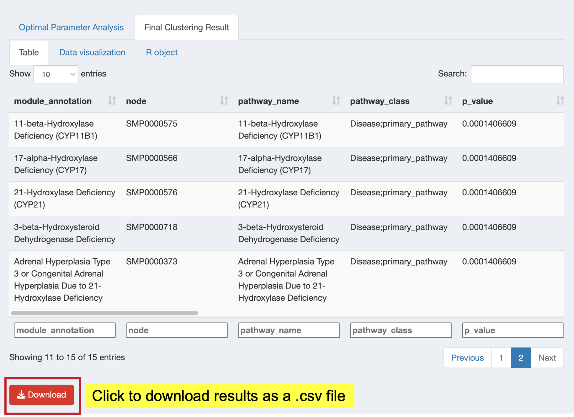
Browse the functional module results and download as CSV:
- View: Complete functional module results table with key metrics
- Download: Click “Download” button to save results as CSV for further analysis
Key result columns:
- module: Functional Module identifier (e.g., “Functional_module_127”)
- module_annotation: Representative pathway name (lowest p-value for ORA, highest |NES| for GSEA)
- Description: Names of all pathways in the module (separated by
;) - module_content: All pathway/term IDs grouped in this module
- Count: Number of genes/metabolites from input list in the module
- p_adjust: Best (lowest) adjusted p-value among pathways in the module
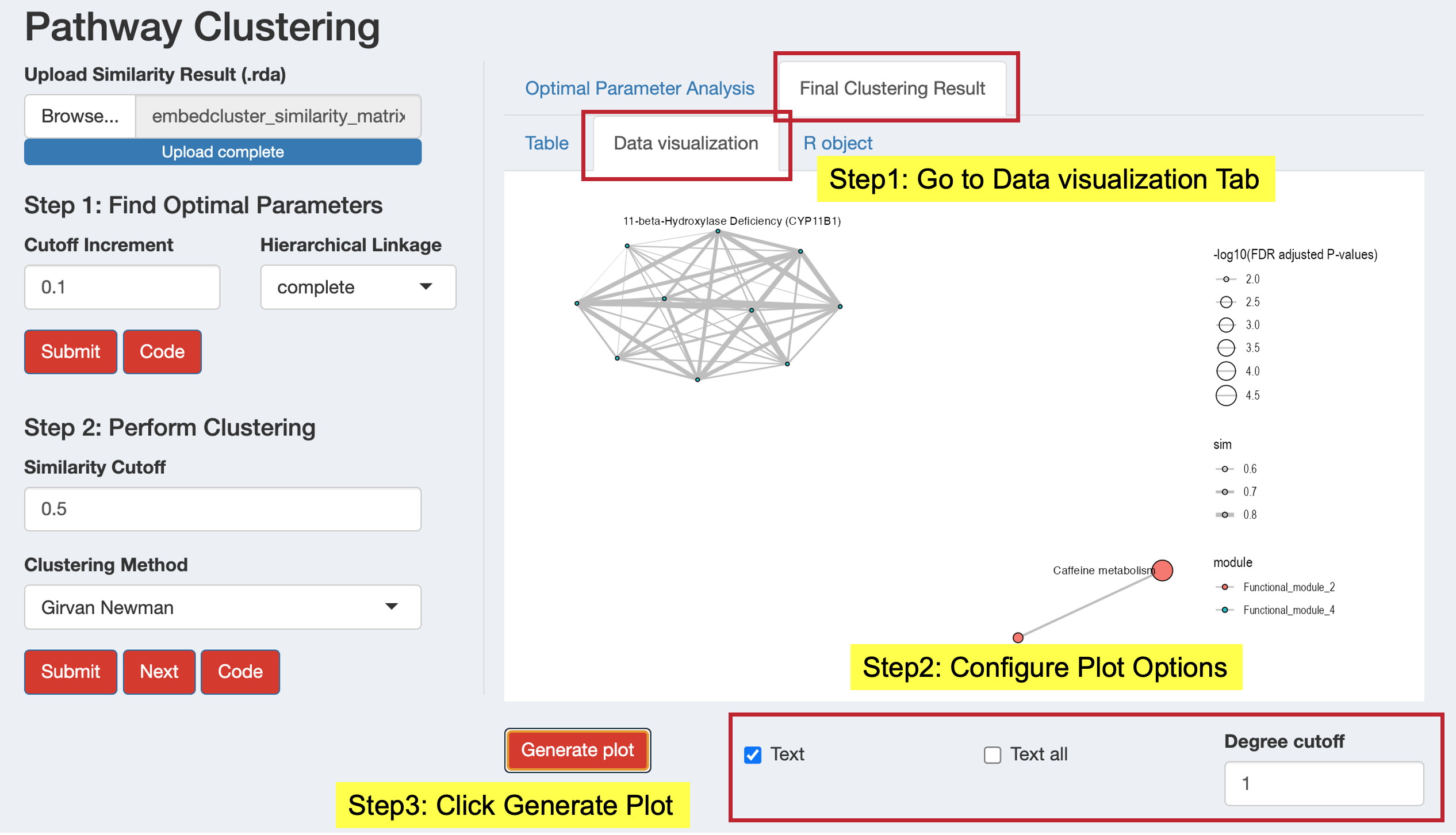
Generate similarity network plots to visualize functional modules:
- Configure plot parameters:
- Degree cutoff: Minimum pathways per module to display
- Text: Show representative module names
- Text all: Show all pathway names
- Click “Generate plot” to create the network visualization
- Examine the network to understand module relationships and structure
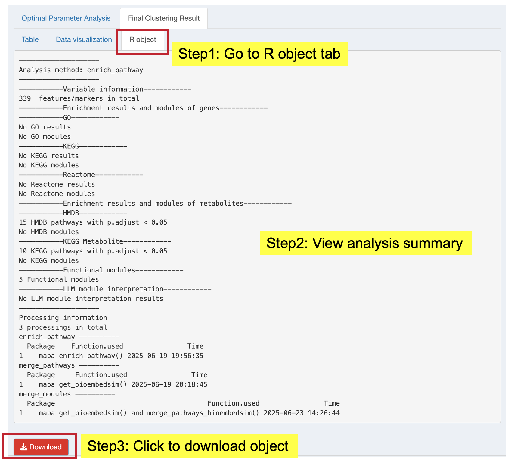
Access the complete results object for further analysis:
- View: Summary of the complete functional module analysis
- Download: Save the complete object (.rda format) for use in R
14.5 Step 4: Assess Clustering Quality
Use the Quality assessment panel to inspect:
Module size: Distribution of module sizes. Avoid many singletons or one giant module.
Silhouette scores: Higher values indicate better cluster separation.
Quality metrics table: Tabular metrics summarizing clustering quality. You can download results; plot Width/Height controls are available where applicable.
You can upload a module identification result (.rda) here if you ran clustering elsewhere and only want to assess quality.
14.6 Step 5: View Analysis Code
Click the “Code” button to see the exact R code that replicates your analysis:
- Module Identification Code: Shows the code used for clustering with your chosen algorithm and cutoff
- Quality Assessment Code: Shows code used to generate size distribution, silhouette plots, and the metrics table
This code can be copied and used in your own R scripts for reproducible analysis.
14.7 Next Steps
Once your functional module identification is complete:
- Download Results: Save both the table and R object for backup and further analysis
- Proceed to LLM Interpretation: Click the “Next” button to move to LLM Interpretation for AI-powered functional annotations of your modules
The functional modules will automatically be available for the next step in your MAPA analysis workflow, where you can add biological context and interpretations using large language models.